

In the previous post, I wrote about the need to structure experiments in a very specific way to keep your results trustworthy. In this post, I’m going to talk about how to structure the experiment results themselves to maximize the value you get from each test.
Say you run an experiment comparing message A with message B. The most common question to ask in these situations is “which message performed better?” That’s not exactly a bad question, but it is a sloppy one. The “which performed better” question limits our experiment to only saying something about the treatments within that one experiment. It yields no information about individual customers (particularly those who didn’t participate in the test), and it gives us no basis for connecting all of learnings from experiments across time.
Every question we could ask after running an experiment basically boils down to “therefore, what?” If you’re running a business, you want your therefores tied directly to business decisions you can make going forward, not to the business decisions you made to produce the therefores in the first place. As long as we report experiment results in relation to the experiment’s treatments and treatment groups, we’re stuck having to spend a lot of time figuring out how to get value out of our results. An experiment isn’t valuable until its results are connected to customers and to other experiments.
Connect experiments to individual customers
So our first task is to take the results of an experiment and say something about each of our customers individually. A customer’s response to any particular message experiment is based on a few things:
Baseline propensity. This is the extent to which a customer is influenced to take the desired action regardless of any experiment conditions. We can measure baseline propensity directly - that’s what we condition experiments. By transforming customer data into latent-space components , we get a compact representation of everything we knew about customers before we introduced them to the experiment. The more we can predict a customer’s action based only on these components, the higher that customer’s baseline propensity to take that action.
Treatment exposure. This is the extent to which a customer is influenced to act because of the treatment condition(s) involved in the experiment. We can also measure treatment exposure directly - that’s the point of the experiment. The more we can predict a customer’s action based on exposure to a particular combination of treatment conditions, the higher those treatments’ influence on that customer’s action.
Other (unknown) influences. People are complicated enough that we can expect their behavior to be influenced by a lot of things we can’t measure or even know about.
We can’t measure these influences directly - by definition, they’re unknown. We can, however, estimate how much unknown influence there is. If we predict customer actions based on both baseline propensity and treatment exposure, we’re going to get some predictions wrong. The fewer predictions we get wrong, the more certainty we have that we’ve captured information about all of the influences that elicited the behavior.
Connect individual customers to future experiments
The point of doing all this is not to say “message A worked better than message B”. It’s to say, for each customer individually, “the next time you have to choose between A and B, here’s how the odds are weighted.” The only reason you run an experiment in a business is because you want that information to inform a future decision. So our experiment results should set us up to make those decisions. What we’re looking for is a “treatment propensity”: the extent to which we can expect a customer to engage in an action because they are exposed to a treatment rather than because they are already predisposed to engage in the action.
We can accomplish this by using machine learning to predict customer actions. Machine learning allows us to consider all of the ways treatments interact with certain baseline propensities and with other treatments to influence outcomes (because it’s usually not as simple as “people with high incomes exposed to treatment A responded more”).
By training a model of the desired behavior that leverages both our latent-space information as well as our treatment assignments, we can estimate the probability that a customer will respond to a treatment, and also measure the extent to which that probability estimate is dependent upon the treatment rather than the latent space information.
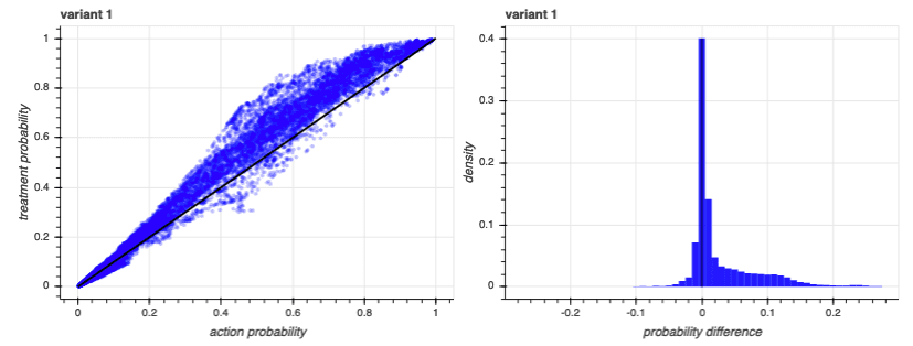
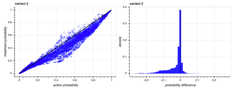
For example, are the results from an experiment that had two variants - we’ll just call them “variant 1” and “variant 2”. In each case, we tried to get participants to do something - in this case, response to a call to action. The percentage of people who responded to that call to action was our success rate. Variant 1 had a 7% success rate and variant 2 had a 3% success rate. Now look at the graphs below:


On the graphs in the left column, we’ve plotted each participant’s baseline propensity prediction along the x-axis, and we’ve plotted each participant’s prediction considering both their treatment exposure and baseline propensity along the y-axis. Participants that fall on the diagonal black line saw no improvement in their predictions by having the model consider treatment exposure. Dots above the diagonal saw an increase in predicted propensity, and dots that fall below the diagonal saw a decrease.
The graphs in the right column show the distributions of the differences in the two scores - the distance from the diagonal black line in the left-column plots. As you can see, the lift in predictions due to specific treatments correlated with the baseline propensity predictions, but only roughly. There are participants who have a baseline prediction of 0.3 whose prediction after incorporating a treatment increases just as much as participants who had a baseline prediction of 0.65. What matters is the increase from baseline, not the actual prediction.
All of this allows us to take the probability of an action given baseline propensity, and probability of action given baseline propensity and treatment exposure, and calculate the probability of action given the treatment. We can estimate, for each individual, how strongly they react to the treatment after discounting the part of the reaction that was due to baseline propensity.
We can see how this works by looking at another experiment. Like the first experiment, this has the same number of treatments, each with the same response rates as the last. But this time, the responses correlate strongly with one of the latent-space components:
Notice that, in this case, many of the baseline predictions are much higher than we had with the first experiment. That’s because the model takes advantage of all available information and, in this case, one of the latent-space components was particularly informative. However, that baseline propensity was so informative that adding in the treatments didn’t really make a difference - the action was one that certain people were likely to engage in anyway, regardless of treatment. We can see that in the distribution plots to the right: almost all of the differences are at or near zero.
So we can use the difference in predictions to estimate the probability that an individual customer will react to a particular treatment. That’s information that is immediately useful for future decisions about each customer.
Connect experiments across time
Now imagine you run the same variant over multiple experiments, each time running it against a different alternative. The probability that a customer reacts to that treatment will change over time. For example, in the two experiments discussed above, variant 1 tended to show a positive impact over the baseline while variant 2 predictions actually tended to fall below the baseline predictions. That’s because variant 1 just generally outperformed variant 2. If we ran variant 2 in a new experiment, against a variant 3, and variant 3 performed worse, the individual reaction probabilities for variant 2 would tend to fall above the baseline. So we need a way of incorporating all of our lessons learned over time to get an estimate of how likely a customer is to react to a particular kind of treatment in general.
That requires us to estimate the quality of the model we use to explain the experiment - a way to quantify how certain we are that the outcome was due to treatment exposure and not to baseline propensity or other influences. Our experiments have binary outcomes: either the customer did the thing we wanted them to do, or they didn’t. When dealing with binary outcomes, I prefer to look at two different metrics:
Precision. If you expose a customer to a treatment because you expect that treatment to cause them to act, and then they don’t act, you’ve wasted effort. Precision measures how well you avoid wasted effort. The lower your precision, the fewer customers acted when exposed to a treatment when your model said they should have acted.
Recall. If you don’t expose a customer to a treatment because you don’t expect that treatment to cause them to act, but they really would have acted if treated, then you’ve missed an opportunity. Recall measures how well you avoid missed opportunities. The lower your recall, the fewer customers who acted your model was able to identify.
However, as with individual predictions, we aren’t primarily concerned with the precision and recall of the model. We’re concerned with the difference in precision and recall between a model that assumes no treatment and a model that assumes a particular treatment. For example, from our first experiment:

These are estimates of precision and recall on different subsamples of our experiment participants. We subsample several times because it helps us see how much our model performance is based on sampling error. The base model uses only our latent-space components to predict an outcome. The full model uses baseline propensity plus treatment exposure.
As you can see, base model precision is around 0.5 and full model precision is around 0.6. Full model recall is around 0.6 to 0.7, but base model recall is very sensitive to random error - it ranges from 0.2 to 0.8.
We can use the distribution of these subsampled scores to estimate the probability that the model with treatment exposure outperforms the baseline propensity model. The full model has an average precision estimate of 0.64, but every one of its precision estimates is higher than every one of the base model estimates. That means it has a 100% chance of performing better. Likewise, the full model has an average recall of 0.67 but a 0.79 chance of achieving better recall than the base model.
We can now look at our second experiment to see how these metrics behave differently when the outcome depends less on treatment exposure and more on baseline propensity:

In this experiment, the full model has a higher average precision and recall - around 0.83 and 0.90 respectively, but these metrics have a lower probability of outperforming the base model: a 0.72 chance for precision and a 0.74 chance for recall.
We can combine these metrics into an overall model certainty score. The score reflects our confidence that treatment exposure has an impact on the outcome, discounted by the gap between the model’s predictive ability and a perfect prediction. That gap is our estimate of all the other, unknown, influences upon the outcome.
Each model’s uncertainty estimate can then act as a weight when combining individual model predictions over time. This way, we can measure a treatment’s performance in a lot of different contexts and make use of all of that information when making our decision about what to do next.
Risk-adjusted success rates
All of the above sets us up to continuously feed results from previous experiments into subsequent experiments, and also creates a wealth of individualized metrics that can be used outside of the experimentation process entirely. As customers are exposed to treatments of varying channels, contact times, value propositions, and incentives, every customer in your database will receive a score estimating how likely they are to respond to those influences. That information can be used in experiments, but it can also be used for segmentation and other business analyses.
None of the above keeps us from getting the traditional answer of “which message performed better.” In fact, it allows us to estimate our success rates in a way that differentiates overall success from attributable success: the success rate that is due to the treatments rather than to baseline propensity. For example, in both examples we used, the success rates were the same: variant 1 had a success rate of 7% and variant 2 had a success rate of 3%. In the first example, the risk-adjusted rates were 3.5% and 1.6% respectively. In the second example, where much more of the success correlated with baseline propensity, the adjusted success rates for the two variants were 1.7% and 0.7% respectively.
Connected experiments move you out of questions about the experiment and immerse you in questions - and answers - about your customers and your business. The results from a connected experiment are immediately actionable. You don’t have to figure out what to do with the results of a connected experiment. The results themselves are next-steps.